
Abstract
Vision-language-action models (VLAs) are moving rapidly towards deployment as general-purpose manipulation policies, but we currently lack basic tools for understanding what these models represent internally or for monitoring them at runtime. Leveraging ideas from mechanistic interpretability, we probe the residual stream of \(\pi_{0.5}\) and find that task progress, the normalized time remaining in a trajectory, is linearly readable from the activations. We find that this signal is present in the pretrained PaliGemma backbone prior to training on any robot-specific data. A single linear probe generalizes to unseen tasks and varies under language counterfactuals when trained on multi-prompt data, but does not enable meaningful steering of the policy. These properties make the signal directly useful for instrumenting deployed VLAs. We use the probe as a simple label-free OOD detector, which detects stalled task progress, and find it competitive with state-of-the-art methods. Our results suggest that VLAs have rich, linearly readable internal representations of semantic quantities like task progress, and that learning to read these signals offers a lightweight, interpretable path toward monitoring deployed visuomotor policies.
Saying that a model "represents" a quantity is ambiguous: it can mean anything from the quantity being recoverable from the activations to the model actually using it to choose its actions. We separate the claim into three concrete, increasingly demanding definitions. We instantiate each on a running example: the target quantity \(\zeta\) is the height of a red mug above the table.
Weak Decodability
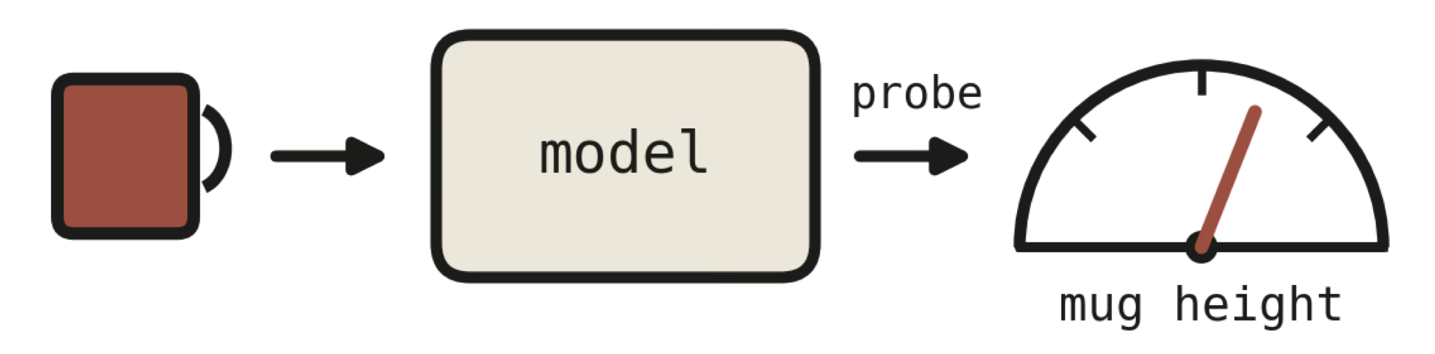
A linear probe \(\varphi\) fit on the frozen model's activations predicts mug height with low error on held-out rollouts. But if the red mug is the only target object in \(\mathcal{D}_{\text{train}}\), a probe reading a correlate of its typical position scores the same.
A quantity \(\zeta\) is weakly decodable from layer \(i\) if the probe attains low risk \(R(\varphi; \mathcal{D}_{\text{val}})\) on validation data drawn from the training distribution. This establishes only that a linear signal correlated with \(\zeta\) can be extracted from in-distribution activations; it does not rule out a spurious correlate standing in for \(\zeta\).
Strong Decodability
To rule this out, we perturb an input factor \(\zeta\) depends on: the prompt is replaced with "pick up the blue bowl," so the target height is now the bowl's. The probe is evaluated unchanged on these transformed inputs. Low error under the swap is inconsistent with the red-mug shortcut.
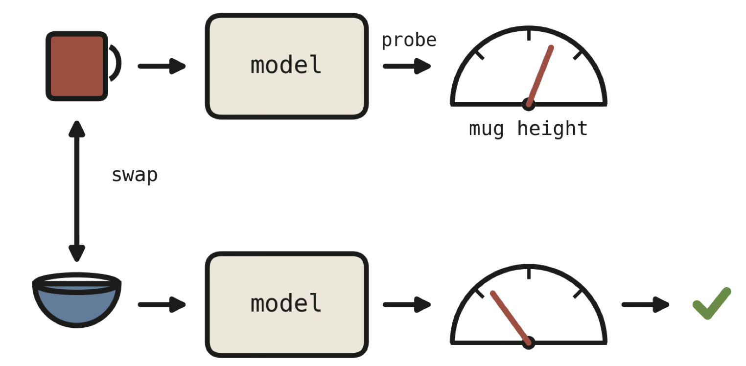
Let \(T:\mathcal{X}\to\mathcal{X}\) be a counterfactual transformation that perturbs the input factors \(\zeta\) depends on, such as \(T_{\text{swap}}\) replacing the prompt \(\ell\) with \(\ell'\). Then \(\zeta\) is strongly decodable if the same probe attains low risk on \(\mathcal{D}_T=\{(z^i(T(x_k)),\, \zeta(T(x_k)))\}_{k=1}^{K}\), i.e. it generalizes to counterfactually transformed inputs without retraining.
Steerability

A strongly decodable signal may still be one the policy does not condition on, so we intervene rather than read. Under \(T_{\text{lift}}\), which raises the mug, we shift the activation along \(w\) until the probe reads the lifted height, and measure whether the resulting action distribution matches the one the true counterfactual induces.
Let \(\pi(z^i)\) be the action distribution when layer \(i\) holds activations \(z^i\). For a counterfactual input \(T(x)\), steer along \(w\):
\[\tilde{z}^i(x) = z^i(x) + \frac{\zeta(T(x)) - \zeta(x)}{\lVert w\rVert^2}\, w\]
so that \(\varphi(\tilde{z}^i)\approx\zeta(T(x))\). With \(\tilde{\pi}_k=\pi(\tilde{z}^i(x_k))\) the steered distribution and \(\pi^\star_k=\pi(z^i(T(x_k)))\) the true counterfactual, the steerability risk is
\[R_S(\varphi;\mathcal{D},T) = \frac{1}{K}\sum_{k=1}^{K} d\!\left(\tilde{\pi}_k,\, \pi^\star_k\right)\]
for a divergence \(d\) between action distributions. Low \(R_S\) means the edit reproduces the behavior the real counterfactual would have produced.
We estimate task progress by fitting a linear probe to \(\pi_{0.5}\)'s residual stream. The policy is left frozen, the regression targets are derived from the rollouts themselves, and the resulting readout requires no forward passes beyond the ones the policy already performs.

- Data collection. We roll out \(\pi_{0.5}\) on manipulation episodes and assign each timestep \(t\) of an episode of length \(T\) the target \(\tau_t = (T - t)/T\), the normalized time remaining. Targets follow from the episode boundaries and require no additional annotation.
- Activation extraction. During each rollout we cache the residual-stream activation \(z^i_t\) at every layer \(i\). Since the probe reads the residual stream rather than a task-specific head, the same procedure applies to the pretrained PaliGemma backbone prior to any robot-specific training.
- Probe training. For each layer we fit \(\varphi(z^i) = w^\top z^i + b\) to \(\tau\). We restrict the probe to be linear so that its accuracy reflects how accessible the quantity is in the representation, rather than the capacity of the probe itself.
- Evaluation. The fitted probe is then assessed for weak and strong decodability, for steerability under activation edits, and as a label-free OOD detector.
Watch the probe track the episode in real time. The trace is the probe's estimate of how much of the task is left, drawn as the rollout plays.
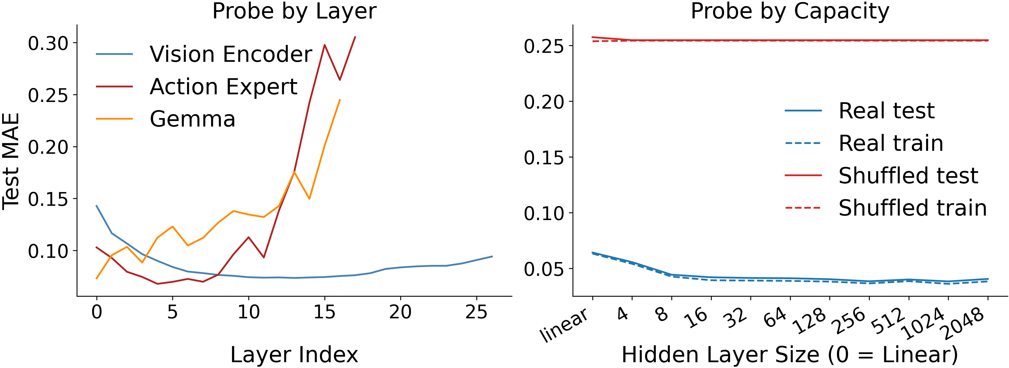
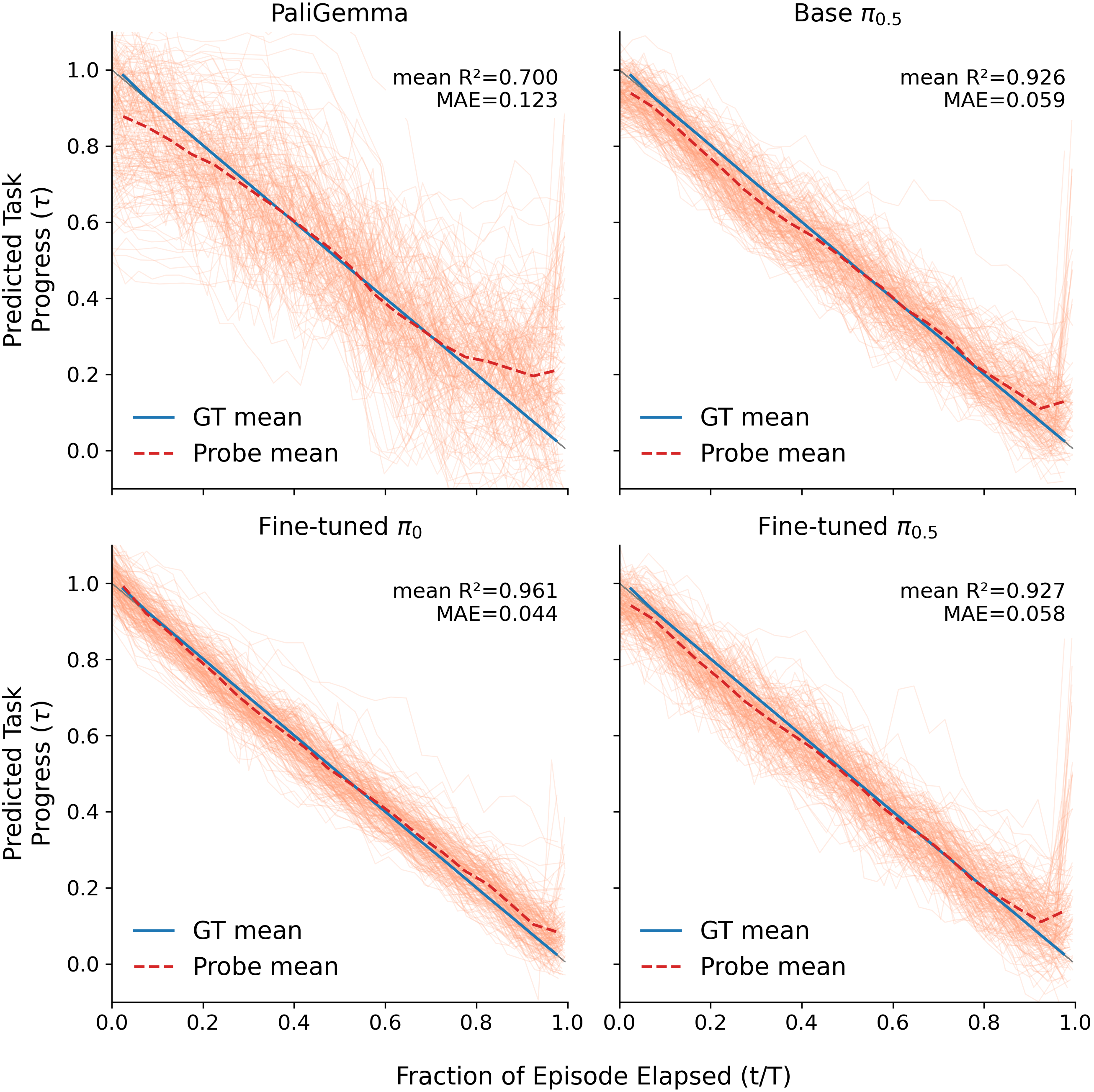
Given these results, task progress is weakly decodable. A plain linear probe reads it from the residual stream with MAE 0.044, the signal is already present in the pretrained backbone before any robot data, and adding probe capacity buys nothing, so the quantity is linearly accessible rather than buried in the activations.
Same episode, same probe, but we swap the target noun in the instruction. A probe that really tracks progress should notice. A naive one doesn't.
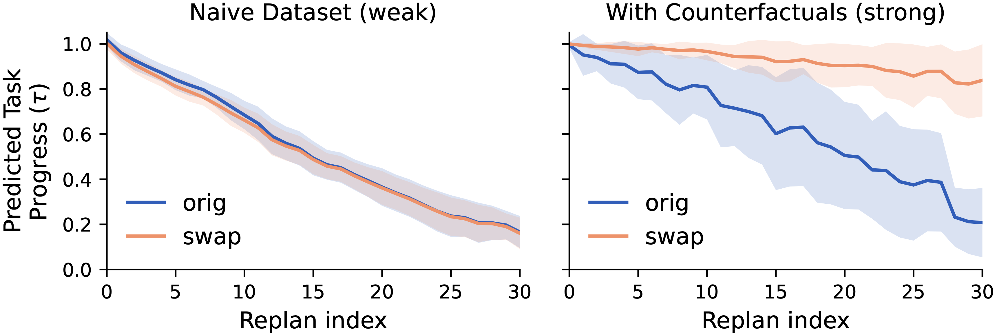
Given these results, task progress is strongly decodable, with counterfactual training data for the probe. A probe fit with counterfactual prompts responds correctly when the instruction changes, while a naively trained probe ignores the swap entirely, so whether the probe tracks the instruction needs counterfactual information during training.
Injecting a boosted progress value along the probe direction does not push the policy toward the behavior that value implies. Progress is readable but not a control handle.
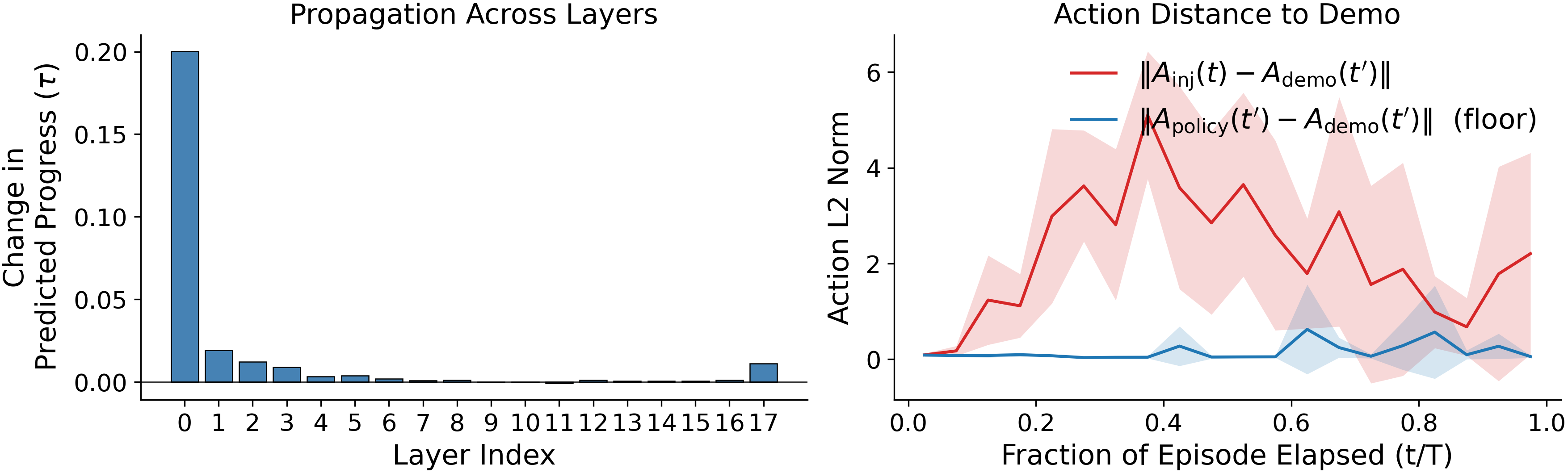
Given these results, task progress is not steerable. The injected value is overwritten within a few layers and the steered actions stay far from the true counterfactual ones, so the policy exposes progress without consulting it when choosing actions. The signal is observable, not a control handle.
In a healthy rollout, task progress falls steadily toward zero. When the policy leaves its training distribution or simply fails, that descent stops. Progress stalls, drifts, or even reverses. The model's own sense of how much is left breaks down at the same moment the episode does, so we can use it as a general failure signal instead of a detector tuned to one kind of corruption.
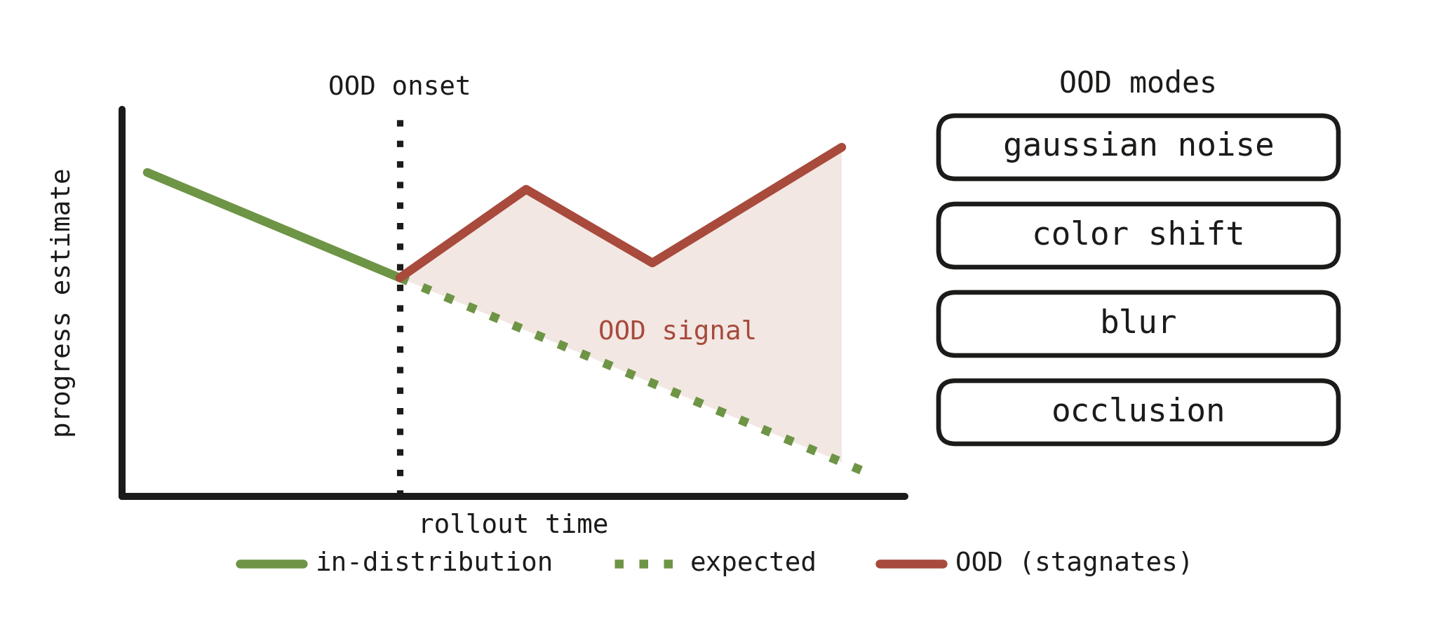
In-distribution, the probe's progress estimate tracks the expected descent. Once the rollout goes OOD (gaussian noise, color shift, blur, occlusion), it stops descending. That stall is the failure signal, and reading it needs no labels.
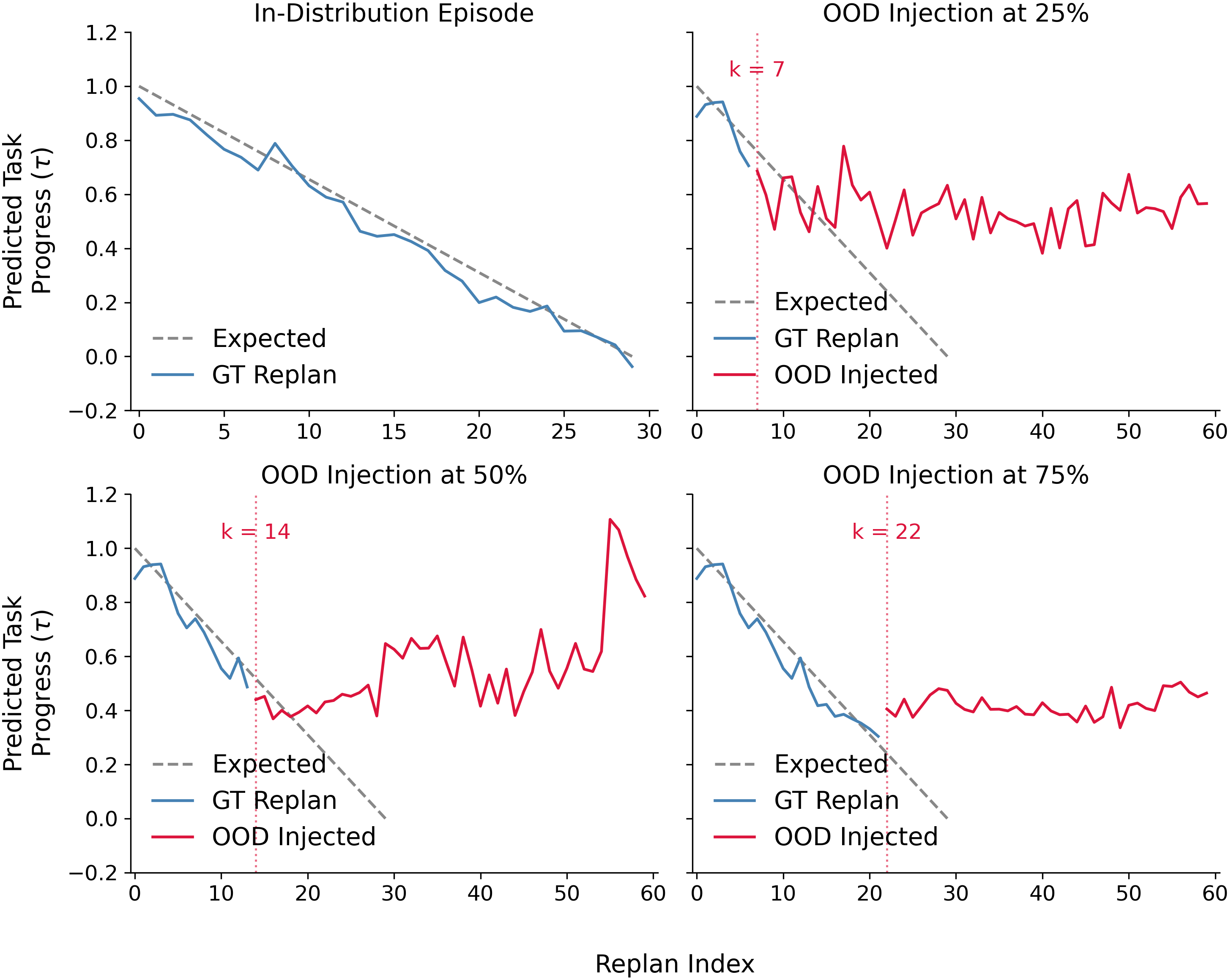
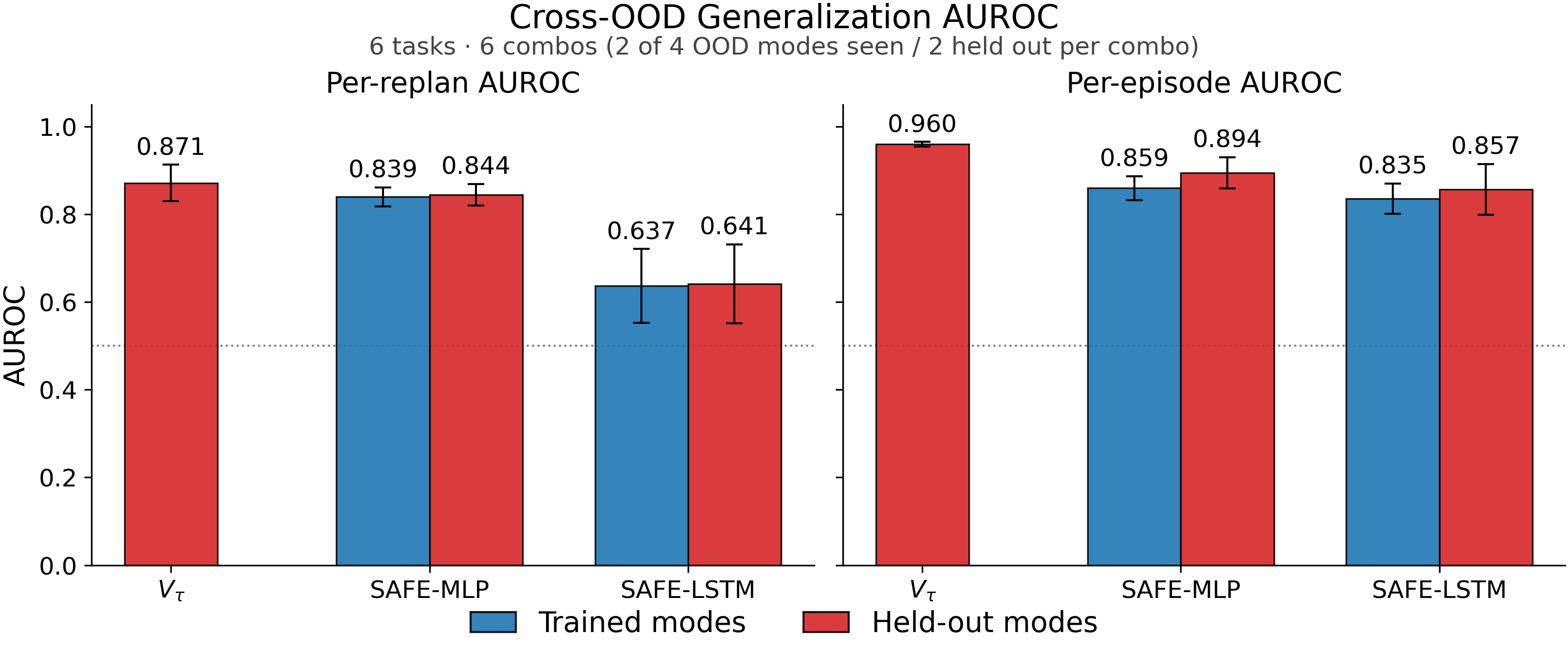
Given these results, the probe makes a practical failure detector. Because progress stalls exactly when a rollout leaves distribution, thresholding the probe's trace flags failures with state-of-the-art AUROC, requires no failure labels, and generalizes to corruption modes it was never tuned on.
Paper
Decoding Task Progress from VLA Representations. Submitted to the 10th Conference on Robot Learning (CoRL 2026).
Read on arXivCode
Probe training, activation extraction, and OOD detection code for reproducing our experiments on \(\pi_{0.5}\) and \(\pi_0\).
Coming soon@inproceedings{bhardwaj2026decoding,
title={Decoding Task Progress from VLA Representations},
author={Bhardwaj, Atiksh and Duan, Edward and Dan, Prithwish and Ma, Wei-Chiu and Culbertson, Preston},
booktitle={Conference on Robot Learning (CoRL)},
year={2026}
}